Phase I Due: Friday, November 8th at class time Phase II Due: Tuesday, November 12th at class time
In this lab, we'll explore the Game of Life. Invented by mathematician John Conway, the Game of Life is what is called a cellular automaton. It is a set of rules rules which are used to generate patterns that evolve over time. Despite the name, the Game of Life is not a game; it is really a simulation. In some ways, it can be thought of as an extremely simplified biological simulator which produces unexpectedly complex behavior.
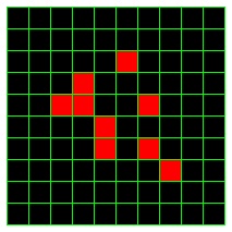
The Game of Life is played on an infinite 2D board made up of square cells. It takes way too long to draw an infinite board, so we'll make due with a small finite piece. Each cell can be either live or dead. We'll indicate a live cell as red, and a dead cell as black. The board begins in some initial configuration, which just mean a setting of each cell to be either live or dead (generally we'll start mostly dead cells, and only a few live cells).
A configuration of a 10-by-10 portion of the board with 9 live cells.
The board is repeatedly updated according to a set of rules, thereby generating a new configuration based on the previous configuration. Some dead cells will become live, some live cells will die, and some cells will be unchanged. This configuration is then updated according to those same rules, producing yet another configuration. This continues in a series of rounds or board-wide steps indefinitely (or until you get bored of running your simulation).
The rules are pretty simple: to figure out whether a cell (c, r) (for column and row) will be live or dead in the following round, you just look at the 8 neighbors of that cell (those that share a corner or an edge, so N, S, W, E, NW, NE, SW and SE). What happens to (c,r) next round depends on the number of its neighbors who are live and whether it is currently live or not. In particular:
For example, consider the following 3 initial configurations, and the two configurations that follow.
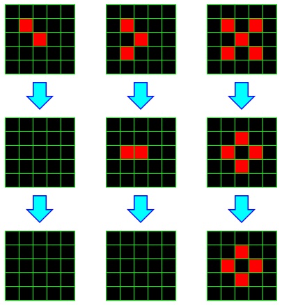
Three initial configurations and two subsequent iterations.
In the first example, both live cells each have only one live neighbor, so they both die. Any dead cell has at most two live neighbors, so no new live cells spawn. Thus in one step, there are no live cells. Clearly, at this point, the configuration has stabilized.
In the second example, two live cells have only one neighbor, so both die. But the third cell lives, and the cell to its immediate left has exactly 3 live neighbors, so it spawns. On the next iteration, we find ourselves in a case similar to the previous example, and all cells die.
In the last example, all currently living cells die; the middle cell has too many neighbors, and the other have too few. However, four dead cells have exactly 3 live neighbors, and so those cells spawn. In the following round, there are neither cells that die nor cells that spawn, so we have a stable configuration. In general, a pattern that doesn't change is called a still-life.
While all of these patterns stabilized quickly, some patterns take a long time to stabilize, and some never do. Of those that never stabilize, some at least have a regularity to them; they eventually repeat states. These are said to be oscillators. Others never repeat the same state again, and produce an infinite number of configurations.
Your first task is to practice (by hand ... with no computer) simulating the Game of Life. Consider the following four initial configurations.
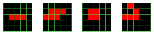
Initial configurations A, B, C and D.
For each of these, you should list the initial configuration and the following four generations of each. To record these, use a fixed width font (like courier) and use a period (.) for a dead cell, and an X for a live cell. For example, the four initial configurations should look like:
..... ..... ..... .X...List below these initial configurations, the next four generations of each in the same format. Also, indicate how many steps it takes for the configuration to oscillate, if it does repeat itself. Be careful: a pattern that appears again in a different location does not count as an oscillator!
Save your solution as life.rtf.
One powerful feature of lists in Python is that you can
have multi-dimensional lists. In class we have been working with two-dimensional lists, or a list of lists. Remember,
A = []
creates an empty list that is referred to by A. The type of the elements of A can be anything, including integers, floats, or strings (which are themselves sequences). So in general, a list named A may have elements that can, themselves be lists.
If we define A to be
A = [ [ 1, 2, 3 ] , [ 4, 5, 6] ]
Then A is a list whose elements are the lists [1, 2, 3] and [4, 5, 6]. We can execute the following in the Python shell once we have the above initialization of A:
>>> A[0]
[1, 2, 3]
>>> A[1]
[4, 5, 6]
In Python, we can treat the elements of a list of lists the same way we treat an individual list, so I can do the following:
A[1].append(7)
A[0].append(-2)
print A
and get:
[[1, 2, 3, -1], [4, 5, 6, 7]]
This notion applies to indexing, slicing, and our other operations on lists, so the following is also available to us:
A[0][2] = -5
to assign the value -5 to the index 2 element of the list given by A[0], so when we print A after this, we would get:
[[1, 2, -5, -1], [4, 5, 6, 7]]
When using this notation, we often call the first index (0 in this case) the row index, and call the second index (2 in this example) the column index. If you wrote A as follows:
A = [[1, 2, -5, -1],
     [4, 5,  6,  7]]
you can see where this terminology comes from. If I want a list of lists of integers associated with variable data with 7 rows and 5 columns, I can generically create and fill such an array with 0 values as follows:
data = [None] * 7
for row in range(7):
    data[row] = []
    for col in range(5):
        data[row].append(0)
In support of our ultimate goal of writing the Game of Life simulation, we are going to focus on writing functions that will serve as building blocks. The first set of functions generically apply to lists of lists of integers. Since we will be using these functions for the board configurations, most of these will have 'board' in the name. For both consistency, and to help by showing how I designed my own functions, I will give the function header and the docstring for the set of general board functions I used in my own solution. As part of Phase I, I want you to design the body of each of these functions. And before you put them into your Game of Life simulation, I want them in a separate Python script called TwoD.py that includes the function definitions along with a main() function definition and invocation that shows ample testing of these functions by themselves.
#-----------------------------------------------------------------------
def createBoard(rows, cols):
    """
    (int, int)-> list of list of ints

    Create a list of list of integers with the given number of
    rows and columns and all elements initialized to 0
    """

#-----------------------------------------------------------------------
def printBoard(board):
    """
    (list of list of ints) -> None

    Traverse the list of lists, whose values are either 0 or 1, printing
    to output, where each 0 prints a '.' and each 1 prints a 'X'. Note
    that you should _NOT_ print lists, but should use nested loops over
    all the elements.
    """

#-----------------------------------------------------------------------
def boardFromFile(filepath):
    """
    (str)-> list of list of ints

    Create a list of list of integers by reading from the file specified
    by the given filepath string. The file will include a header line
    with the number of rows and columns, and then will follow with rows
    lines in the file, each with columns numbers in the line.
    """

#-----------------------------------------------------------------------
def copyBoard(D, S):
    """
    (list of list of ints, list of list of ints)->None

    Perform a two dimensional deep copy of the elements of the given
    source, S, to the given destination, D.
    """
We'll be using all of the function building blocks created above in our Game of Life simulation. So now, let's think about how we might go about setting up our Life simulator. By separating into two phases, we are going to force the professor's advice of working on the core algorithms before we work on the display aspects of the solution (which we will save for Phase II). So in this phase, our user interface will use printing of board configurations to the output window, and will just use the input() and pickAFile() functions to gather necessary information from the user.
Another sound piece of advice is to start simple and then slowly work our way to a more complete solution. In this case, we will start by designing a sequence that will just take a Game of Life board from some initial configuration through exactly one step/generation.
The boardFromFile() function above, along with a call to pickAFile() can allow us to associate a variable, call it board, with an initial configuration, as long as we have created a text file with the desired initial board configuration. Our next task is to apply the Rules above to each of the cells to get a new configuration. But when we think about the job of applying the rules of the simulation to board we should be able to see a problem: if we need to count all the neighbors of a given cell, and then change the value of that cell according to those rules, what happens when we need to perform the same evaluation on a subsequent cell? If we have changed the value of one cell, it no longer represents the information needed for neighboring cells. Our solution is to maintain two versions of the board. The second version of the board, call it boardCopy is a list of lists initialized to zero with the same number of rows and columns as in the original board. Each time we need to update the board (i.e. at each generational step), we first copy the values from board to boardCopy. To update board, for each cell, we count the number of live neighbors by examining the values in boardCopy and use that information to update values in board.
The sequence to accomplish this for our one-step version of the program can be summarized as follows:
All these parts should be straightforward by utilizing the functions defined in Part 2, except for the fifth step. We will try to solve the problem by inventing functions to solve smaller parts of the problem. First, consider a function called countNeighbors() whose job is to count the number of live neighbors of a given row, col cell position in a given board. With the countNeighbors() function, we can envision a function evalCell() that evaluates a single cell by counting the neighbors of a cell and, using that count along with the value (0, 1) of the current cell, yields a 0 or 1 as the new value of a cell. This function could be the core of a function, evalBoard that iterates over all of the internal cells of the copy of the board configuration to update the cells of the board.
As with the general board functions above, I am going to provide the function header and docstring for these three functions and your task is to fill in the body of each of these three functions:
#-----------------------------------------------------------------------
def countNeighbors(B, row, col):
    """
    (list of list of ints, int, int)->int

    For row > 0 and row < len(B)-1, and col > 0 and col < len(B[0])-1,
    return the integer count of the number of live cells in the
    eight neighbors surrounding the cell at B[row][col].  The caller
    is responsible for enforcing the constraint that we can only count
    neighbors of the _internal_ cells of B.
    """

#-----------------------------------------------------------------------
def evalCell(B, row, col):
    """
    (list of list of ints, int, int)->int

    Evaluate a single cell in board B, based on the rules of Life.
    The cell to evaluate is given by the row, col parameters.  The return
    is either 0 if the evaluation results in a dead cell, or 1 if the
    evaluation results in a live cell.
    """

#-----------------------------------------------------------------------
def evalBoard(past, next):
    """
    (list of list of ints, list of list of ints) -> None

    Iterate over all the _internal_ cells of the board given by past,
    invoking the evalCell() function for past at each row, col pair
    and updating the board, next, with the obtained value.
    """
One caution that is part of the above docstring comments: In this first version of the game, (particularly in evalBoard()), our loops are not iterating over all the cells in the board. These loops should be restricted to the internal cells of the board. The reason for this is simple: we have not defined what the "northerly" neighbors of row 0 should be. Nor the "southerly" neighbors of the bottom row, the "westerly" neighbors of the first column, and the "easterly" neighbors of the last column. We simplify by avoiding the problem and only computing evaluations on the internal cells.
Time to assemble all the pieces. Use the steps outlined in Part 3, realized by the functions developed in Part 2 and in Part 4 to get your program to read in an initial configuration, print it out, and then take a single step of the simulation, and then print out the result. By creating a good set of files to use as the initial configuration, you can debug the algorithms of your Game of Life simulation to make sure they all work correctly. Assemble this one-step version into a program called LifeOneStep.py and include at least a half dozen initial configurations to demonstrate that you have tested it well.
Now it is time to take multiple steps. After getting the initial board configuration file from the user and initialing the board, printing the board, and creating the board copy, we can then use the input() function to ask the user how many steps they want to take. If the user enters 0, the program is finished. If the user enters a positive integer, then the program will repeatedly:
The print/output window and minimal user interface version of the Game of Life lacks the visual satisfaction of a graphically oriented solution. The purpose of Phase II, now that we have a (hopefully) working set of functions and algorithms, is to remedy that deficiency.
The most basic form of user interface would use a Calico Window for displaying the cells of a board. Whenever we invoke printBoard() in the non-UI version of the game, we will instead call a displayBoard() function ... so at each iteration of the high-level generation loop, after a board configuration is updated. Given a list of lists of 0/1 integers specifying a board configuration, displayBoard() will update the Window created during initialization with the Graphics operations to display the given board.
When we consider how to map the Life board cells to a display window, we can see that we will want each cell of the board to correspond to a Rectangle object arranged in a grid in the window. Each such Rectangle can be filled with a color that corresponds to the cell being "alive" or "dead". In the examples above, we use a fill color of black for a dead cell and red for a live cell.
As implementation guidance, let us consider the work we need to do one time as part of initialization versus what we need to do as we iterate over generational steps during the simulation.
#-----------------------------------------------------------------------
def createGrid(rows, cols, win):
	"""
	(int, int, Window) -> list of lists of Rectangles

	Using tileSize and row/col indices, create a list of lists of Rectangles
	drawn in the given Window, win.  There should be rows rows and cols cols in the
	list of lists, and the Rectangles should be distributed in a grid over
	the Window.
	"""
#-----------------------------------------------------------------------
def displayBoard(grid, board):
	"""
	(list of lists of Rectangles, list of lists of ints) -> None

	Iterate over all Rectangle elements of grid, using the corresponding
	element of board such that, whenever the element of board contains a
	0, update the fill color of the corresponding Rectangle with the black
	color, and whenever the element of board contains a 1, update the fill
	color of the corresponding Rectangle with the red color.
	"""
import timeThen, we can invoke the sleep function by naming the module, and calling the sleep function with an argument that specifies the time, in seconds, for the program to delay. IF we want a delay of a half second, that would look like the following:
time.sleep(0.5)
Per usual, I encourage you to make improvements to make a nicer user experience. One could imagine a number of enhancements. For instance, the solution above assumes that, for any initial board configuration, the size of each square in the window is the same. This limits the size of a board. The program could instead assume a maximum width and height of the display window and then compute the tileSize based on the initial board configuration ... so a small board would result in bigger squares and a large board would result in smaller squares.
The user interface could also be enhanced with a button that, when pressed, determines a new number of steps for the program to iterate through. Or a button that allows free-running. Or a button that allows, from within the program, a reset and reading a new board.